3 Linear Regression
3.1 Definition
Suppose that a random sample of size \(n\) is drawn from a population, and measurements \((x_{i1}, x_{i2}, \dots, x_{ik}, y_i)\), where \(i = 1, \dots, n\), are obtained on the \(n\) individuals.
The random variables \(x_{i1}, x_{i2}, \dots, x_{ik}\) are commonly termed predictor variables (or simply, predictors). Depending on the field of application, they may also be called independent variables, regressors, features, covariates, or explanatory variables.
The \(y_i\) variable is called the response variable (or simply, response). Other terms include target variable, variate, dependent variable, or outcome variable.
The Linear Regression Model represents a relation between the response variable \(y\) and the predictor variables \(x_1, x_2, \dots, x_k\) (with lowercase notation for simplicity), of the form:
\[ y = \beta_0 + \beta_1 x_1 + \beta_2 x_2 + \dots + \beta_k x_k + \epsilon \]
Where \(\beta_0, ..., \beta_k\) are constants regression coefficients, and \(\epsilon\) is a random error term that follows a normal distribution with mean zero (\(\mu = 0\)) and constant variance \(\sigma^2\). That is, \(\epsilon \sim Norm(\mu = 0, \sigma^2)\). Also, the random errors are assumed to be independent for different individuals of the sample.
The parameters of the model \(\beta_0, ..., \beta_k\), and the variance \(\sigma^2\) are unknown and have to be estimated from the sample data.
Note that the relationship between the predictors and the response is not necessarily linear, as polynomial or interaction terms may be included, but it is necessarily linear in the beta coefficients. That is, the relationship is modeled as a linear combination of the parameters.
Note that, in the general linear regression model, the response variable y has a normal distribution with the mean:
\[ \begin{align} \mathbb{E}(y|x) = \beta_0 + \beta_1 \cdot x_1 + ... + \beta_k \cdot x_k \end{align} \]
3.2 Simple Linear Regression
Simple linear regression is a simplification of the Linear Regression Model that estimates the relationship between one independent variable and one dependent variable using a straight line. Both variables should be quantitative.
For this example, we’ll use the Boston dataset, which contains 506 census tracts in Boston. We will seek to predict medv, the median house value, using the lstat predictor, which represents the percent of households with low socioeconomic status.
##      crim zn indus chas   nox    rm  age    dis rad tax ptratio lstat medv
## 1 0.00632 18  2.31    0 0.538 6.575 65.2 4.0900   1 296    15.3  4.98 24.0
## 2 0.02731  0  7.07    0 0.469 6.421 78.9 4.9671   2 242    17.8  9.14 21.6
## 3 0.02729  0  7.07    0 0.469 7.185 61.1 4.9671   2 242    17.8  4.03 34.7
## 4 0.03237  0  2.18    0 0.458 6.998 45.8 6.0622   3 222    18.7  2.94 33.4
## 5 0.06905  0  2.18    0 0.458 7.147 54.2 6.0622   3 222    18.7  5.33 36.2
## 6 0.02985  0  2.18    0 0.458 6.430 58.7 6.0622   3 222    18.7  5.21 28.7
We will start by using the lm function to fit a simple linear regression model, with medv as the response and lstat as the predictor. The basic syntax is lm(y ∼ x, data), where y is the response, x is the predictor, and data is the data set (usually a dataframe) in which these two variables are kept.
linear_reg <- lm(formula = medv ~ lstat, data = df)If we type the name of the variable, which in this case is linear_reg some basic information about the model is output.
linear_reg##
## Call:
## lm(formula = medv ~ lstat, data = df)
##
## Coefficients:
## (Intercept) lstat
## 34.55 -0.95For more detailed information, we use summary(linear_reg). This gives us p-values and standard errors for the coefficients, as well as the \(R^2\) statistic and \(F\)-statistic for the model.
summary(linear_reg)##
## Call:
## lm(formula = medv ~ lstat, data = df)
##
## Residuals:
## Min 1Q Median 3Q Max
## -15.168 -3.990 -1.318 2.034 24.500
##
## Coefficients:
## Estimate Std. Error t value Pr(>|t|)
## (Intercept) 34.55384 0.56263 61.41 <2e-16 ***
## lstat -0.95005 0.03873 -24.53 <2e-16 ***
## ---
## Signif. codes: 0 '***' 0.001 '**' 0.01 '*' 0.05 '.' 0.1 ' ' 1
##
## Residual standard error: 6.216 on 504 degrees of freedom
## Multiple R-squared: 0.5441, Adjusted R-squared: 0.5432
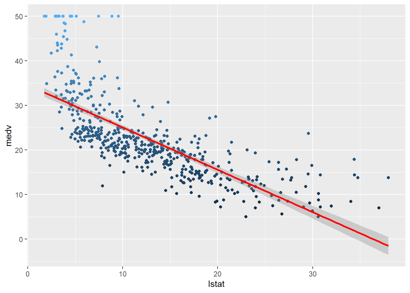
## F-statistic: 601.6 on 1 and 504 DF, p-value: < 2.2e-16We can also plot the linear regression line using ggplot2:
ggplot(data = df,
       mapping = aes(x = lstat,
                     y = medv,
                     col = medv)) +
  geom_point() +
  geom_smooth(method=lm, formula = y ~ x, col="red") +
  guides(col="none")
3.3 Polynomial Regression
It is also possible to fit a polynomial regression model by using the poly function, whose first argument is the variable and the second is the degree of the polynomial.
##
## Call:
## lm(formula = medv ~ poly(lstat, 2), data = df)
##
## Coefficients:
##     (Intercept)  poly(lstat, 2)1  poly(lstat, 2)2
##           22.53          -152.46            64.23
It is also possible to print the summary of the model, by using the aforementioned summary function.
summary(polynomial_reg)##
## Call:
## lm(formula = medv ~ poly(lstat, 2), data = df)
##
## Residuals:
## Min 1Q Median 3Q Max
## -15.2834 -3.8313 -0.5295 2.3095 25.4148
##
## Coefficients:
## Estimate Std. Error t value Pr(>|t|)
## (Intercept) 22.5328 0.2456 91.76 <2e-16 ***
## poly(lstat, 2)1 -152.4595 5.5237 -27.60 <2e-16 ***
## poly(lstat, 2)2 64.2272 5.5237 11.63 <2e-16 ***
## ---
## Signif. codes: 0 '***' 0.001 '**' 0.01 '*' 0.05 '.' 0.1 ' ' 1
##
## Residual standard error: 5.524 on 503 degrees of freedom
## Multiple R-squared: 0.6407, Adjusted R-squared: 0.6393
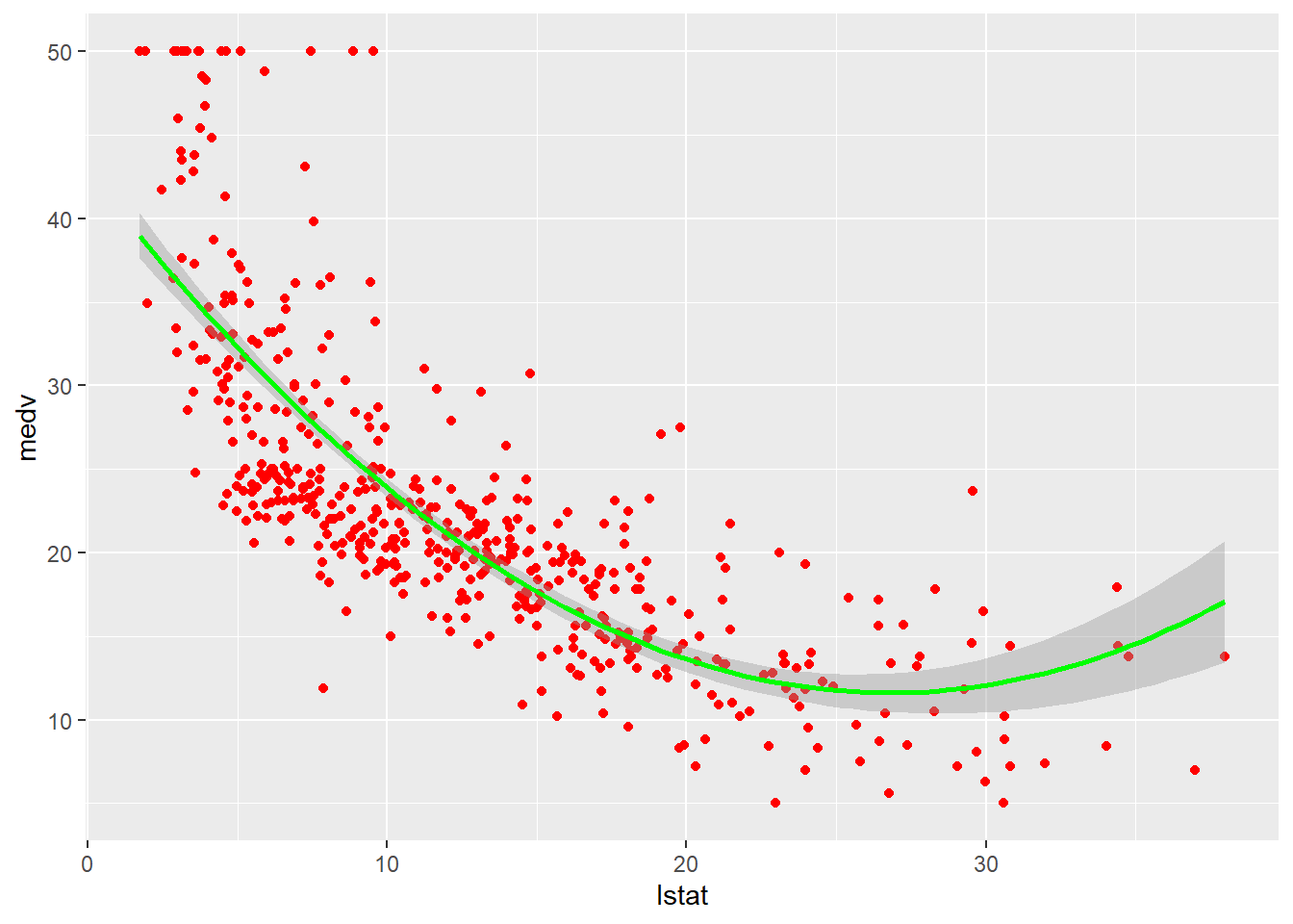
## F-statistic: 448.5 on 2 and 503 DF, p-value: < 2.2e-16Similarly, we can plot this polynomial regression model using ggplot2:
ggplot(data = df,
       mapping = aes(x = lstat,
                     y = medv,
                     col = medv)) +
  geom_point(col="red") +
  geom_smooth(method=lm, formula = y ~ poly(x, 2), col="green") +
  guides(col="none")
3.4 Multiple Linear Regression
We will continue to use the Boston dataset in order to predict medv using several predictors such as rm (average number of rooms per house), age (average age of houses), and lstat (percent of households with low socioeconomic status).
In order to fit a multiple linear regression model using least squares, we again use the lm function. The syntax lm(y ∼ x1 + x2 + x3) is used to fit a model with three predictors, \(x_1\), \(x_2\), and \(x_3\). The summary function now outputs the regression coefficients for all the predictors.
##
## Call:
## lm(formula = medv ~ lstat + age, data = df)
##
## Residuals:
##     Min      1Q  Median      3Q     Max
## -15.981  -3.978  -1.283   1.968  23.158
##
## Coefficients:
##             Estimate Std. Error t value Pr(>|t|)
## (Intercept) 33.22276    0.73085  45.458  < 2e-16 ***
## lstat       -1.03207    0.04819 -21.416  < 2e-16 ***
## age          0.03454    0.01223   2.826  0.00491 **
## ---
## Signif. codes:  0 '***' 0.001 '**' 0.01 '*' 0.05 '.' 0.1 ' ' 1
##
## Residual standard error: 6.173 on 503 degrees of freedom
## Multiple R-squared:  0.5513, Adjusted R-squared:  0.5495
## F-statistic:   309 on 2 and 503 DF,  p-value: < 2.2e-16
The Boston data set contains 12 variables, and so it would be cumbersome to have to type all of these in order to perform a regression using all of the predictors. Instead, we can use the following short-hand:
##
## Call:
## lm(formula = medv ~ ., data = df)
##
## Residuals:
##      Min       1Q   Median       3Q      Max
## -15.1304  -2.7673  -0.5814   1.9414  26.2526
##
## Coefficients:
##               Estimate Std. Error t value Pr(>|t|)
## (Intercept)  41.617270   4.936039   8.431 3.79e-16 ***
## crim         -0.121389   0.033000  -3.678 0.000261 ***
## zn            0.046963   0.013879   3.384 0.000772 ***
## indus         0.013468   0.062145   0.217 0.828520
## chas          2.839993   0.870007   3.264 0.001173 **
## nox         -18.758022   3.851355  -4.870 1.50e-06 ***
## rm            3.658119   0.420246   8.705  < 2e-16 ***
## age           0.003611   0.013329   0.271 0.786595
## dis          -1.490754   0.201623  -7.394 6.17e-13 ***
## rad           0.289405   0.066908   4.325 1.84e-05 ***
## tax          -0.012682   0.003801  -3.337 0.000912 ***
## ptratio      -0.937533   0.132206  -7.091 4.63e-12 ***
## lstat        -0.552019   0.050659 -10.897  < 2e-16 ***
## ---
## Signif. codes:  0 '***' 0.001 '**' 0.01 '*' 0.05 '.' 0.1 ' ' 1
##
## Residual standard error: 4.798 on 493 degrees of freedom
## Multiple R-squared:  0.7343, Adjusted R-squared:  0.7278
## F-statistic: 113.5 on 12 and 493 DF,  p-value: < 2.2e-16
3.5 Wilkinson-Rogers Notation
The feature of detailing all variables by using a . placeholder is possible because R uses Wilkinson and Rogers’ (1973) notation, which allows us to write the algebraic formula that defines a statistical model.
This notation is commonly used in R, Python & MATLAB statistical libraries.
Below is a table in which the symbols that helps write formulas to represent statistical models appear.
